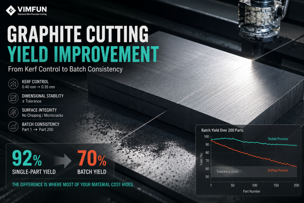
A graphite cutting operation running at 92% single-part yield can easily drop to 70% batch yield across a 200-part production run — the difference is where most of your material cost hides. Graphite cutting yield improvement is not about improving one cut; it is about controlling the variance across every cut in a batch. This page covers why single-part yield never predicts batch yield accurately, the four levers that actually move batch yield (kerf control, dimensional stability, surface integrity, batch consistency), and the diagnostic sequence to use when yield drops instead of blaming material first.
For production and process engineers, cải thiện sản lượng cắt than chì means treating each yield loss as a signal — kerf drift, dimensional fade, surface defects, or fixture wear — and attacking the largest signal first. The following breakdown assumes you already have a Pillar-level understanding of kerf economics from low-kerf graphite cutting; this page picks up where cost framing ends and outcome measurement begins.
Why Graphite Cutting Yield Is Different from Machining Yield
Graphite cutting yield is measured by usable output divided by starting material volume, and unlike metal machining, the material removed by the kerf itself is a permanent, unrecoverable loss. Machining generates chips that carry no reusable geometry; cutting generates two usable parts separated by a kerf, so every millimeter of kerf is measurable material loss.
This distinction matters because yield in a machining context can be recovered through better tool paths or finer finishing passes. In graphite cutting, once the kerf is gone, it is gone — meaning cải thiện sản lượng cắt than chì is bounded by both the physical kerf and the process consistency around it.
Yield is also different from material utilization rate. Utilization measures how efficiently your part geometry fits into the raw block. Yield measures how consistently your process converts that theoretical utilization into shippable parts. A high-utilization design with poor process control still delivers low yield.
Yield Lever 1: Kerf Control
Kerf loss directly bounds the maximum theoretical yield of any graphite cutting operation. If your kerf averages 0.4mm on a slicing job with 5mm target parts, roughly 8% of your material is permanently locked in kerf loss before any other variable enters the equation.
The nuance: kerf reduction alone rarely improves yield significantly if your process is inconsistent. Reducing average kerf from 0.4mm to 0.35mm looks like a 12% kerf improvement, but if your kerf standard deviation is 0.05mm — meaning individual cuts range from 0.30mm to 0.40mm — the actual yield gain is dampened by the parts you scrap due to dimensional drift.
For detailed operational guidance on kerf control, see our companion piece on how to reduce kerf loss in graphite cutting. For cải thiện sản lượng cắt than chì, treat kerf as a necessary but not sufficient lever — reduce it, but always alongside consistency work.
Yield Lever 2: Dimensional Stability Across the Batch
Dimensional stability is often the largest hidden yield lever, especially in operations that already have kerf under control. Cuts that pass first-article inspection can drift out of specification mid-batch as tools wear, fixtures shift, or thermal conditions change.
The typical failure pattern: your first 20 parts hit target dimensions with tight tolerance, but by part 100 your dimensions have shifted 0.1mm one direction, and by part 180 you have drifted enough to trigger dimensional rejections. Your first-article inspection said the process was capable; your batch yield says otherwise.
We saw exactly this failure mode on a slicing job for a customer running isostatic graphite blocks for semiconductor CVD susceptor blanks. First-article measurements looked perfect. The operator ran the batch overnight. By morning, roughly one-third of the parts near the end of the run were 0.08mm oversized — not enough to catch by visual inspection, but enough to fail the downstream grinding allowance. The cause was fixture creep from thermal expansion of the coolant recirculation loop, which we only found by instrumenting the fixture temperature during a repeat run. The fix was a coolant flow adjustment; the lesson was that overnight batches need mid-batch sampling logged against clock time.
Practical stability checks include:
- Mid-batch dimensional sampling — measure every 30–50 parts, not just first and last
- Tool wear tracking — record cumulative cutting time per tool, correlate to dimensional drift
- Thermal monitoring — extended cuts can heat fixtures enough to shift setup by tens of microns
- Post-cut dimensional plots — a scatter plot of dimensions vs part number reveals drift patterns that averages hide
Dimensional stability is where cải thiện sản lượng cắt than chì stops being about the cut and starts being about the manufacturing system around the cut.
Yield Lever 3: Surface Integrity
Surface defects — micro-cracks, chip-outs, edge burrs, and fracture zones — cause yield losses that never appear in dimensional inspection. A part can measure within tolerance but fail visual or downstream integration inspection because of surface issues.
For most graphite grades used in industrial applications, surface integrity depends on the interaction between cutting speed, tool sharpness, and feed rate. Aggressive feeds on softer graphite grades produce chip-outs that render parts unusable for their intended application. Conservative feeds on harder grades may not chip but generate excessive tool wear that later causes dimensional drift — an example of the trade-off that makes yield improvement harder than any single-variable optimization.
Micro-cracks are the hardest to catch because they may not surface until downstream stress or thermal cycling. Some manufacturers accept surface defects at the cutting stage and rely on downstream inspection, but this shifts yield loss from cutting to later stages — the total yield problem does not disappear, it just changes categories. See surface damage in graphite machining for related discussion.
Yield Lever 4: Batch Consistency (The Hidden Killer)
Single-part yield is almost always higher than batch yield, and the delta is where most graphite operations lose money. A process producing 95% good parts on the first 10 cuts can produce 75% good parts by cut 200 — for reasons that are not always obvious in real time.
The drivers of batch yield decay typically include:
| Consistency Factor | Typical Impact on Batch Yield |
|---|---|
| Tool wear (dimensional drift) | 5–15% yield loss over tool life |
| Fixture creep (setup shift) | 3–8% yield loss per batch |
| Coolant contamination or depletion | 2–6% yield loss when coolant is neglected |
| Thermal drift (long production runs) | 2–5% yield loss on extended batches |
| Operator variability (multi-shift ops) | 3–10% yield variance shift-to-shift |
The compounding effect is what makes batch yield so hard to improve. Even a 3% yield loss from each of four factors doesn’t add to 12%; the interactions between factors can push actual loss above 20% for uncontrolled operations. This is also why single-variable optimization campaigns often disappoint — you fix one contributor and the others expand to fill the space.
For batch consistency work, our related discussion of sự ổn định trong sản xuất than chì covers process control fundamentals that apply directly to yield sustainment.
How to Track and Diagnose Graphite Cutting Yield Systematically
Before you can improve yield, you need to measure it in a way that separates signal from noise. The most common mistake in cải thiện sản lượng cắt than chì projects is chasing anecdotal yield problems without a baseline.
Establish a yield baseline (4 weeks of rolling data):
- Define yield precisely — usable shipped parts ÷ starting material volume, not “good parts ÷ total parts”
- Segment by product type — a single yield number hides where the problem lives
- Track daily, review weekly — daily numbers show noise, weekly averages show trends
- Log context — tool changes, operator shift, material batch, fixture setup
When yield drops, diagnose in this sequence:
- Dimensional distribution first — did parts start missing target dimensions, or did they always?
- Surface defect pattern next — new defect type, or same defect at higher rate?
- Kerf drift third — is your kerf drifting mid-batch?
- Fixture and tool wear fourth — cumulative time on both since last replacement
- Material batch last — material variance is real but usually the smallest contributor
The instinct to blame material first is common but often wrong. Reputable graphite suppliers such as SGL Carbon Và Toyo Tanso publish material specifications with tight tolerances; material-driven yield loss usually shows as batch-level shifts, not gradual drift within a batch.
Cost Impact of Graphite Cutting Yield Improvement
A yield improvement of 5% on an operation running 1,000 kg of graphite per month translates to 50 kg of recovered material — but the real cost impact depends on what value density that material carries. Low-grade graphite recovery is measured in tens of dollars per kilogram saved; high-grade isostatic graphite for semiconductor applications can be measured in hundreds.
Yield improvement compounds with kerf reduction. A 5% yield gain combined with 10% kerf reduction on high-value graphite delivers material savings that typically pay back process improvement investments within a fiscal quarter — but only if the process holds long enough for the savings to accumulate. This is why sustainment work (documented procedures, operator training, statistical process control) usually matters more than one-time technical wins.
For purchasing teams evaluating cost trade-offs, the practical implication: a supplier or process offering 3% higher yield at 2% higher cost per hour typically wins on total material cost. Yield economics rarely favor the lowest hourly price. See our P4 Pillar on low-kerf graphite cutting for the full cost-side view.
Realistic Yield Improvement Targets
For operations with basic process control in place, a 3–8% batch yield improvement is a realistic 3-month target through combined kerf control and consistency work. Larger gains typically require equipment or fixture redesign, not just process tuning.
For operations without basic controls (no yield baseline, no dimensional tracking, no tool wear logs), the first 30–60 days should focus on establishing visibility, not chasing gains. Trying to improve what you cannot measure produces false wins and hides real problems.
A practical engineering judgment: if you can only work on one lever this quarter, work on batch consistency, not average kerf. Reducing kerf standard deviation by 30% typically moves yield more than reducing average kerf by 10%. The math is not intuitive, but the field evidence is consistent.
Related Resources for Yield Improvement Work
- Low-Kerf Graphite Cutting Pillar — cost and economic framing of kerf loss
- How to Reduce Kerf Loss in Graphite Cutting — operational how-to for the kerf lever
- Graphite Machining Surface Damage — surface integrity failure modes
- Graphite Manufacturing Stability — process control fundamentals for batch consistency
For occupational safety considerations in graphite cutting operations, refer to OSHA guidelines on respiratory protection for dust exposure.
Câu hỏi thường gặp
What is a good yield rate for graphite cutting?
Yield rates vary by material value and cutting geometry. For high-value graphite in precision applications, batch yield above 85% is generally considered healthy. Below 75% usually indicates a process control issue rather than a material issue. The absolute number matters less than whether your process is stable — an operation running consistently at 82% is easier to improve than one bouncing between 70% and 90%.
Is kerf reduction the same as yield improvement?
No. Kerf reduction is one lever, but yield also depends on dimensional stability, surface integrity, and batch consistency. Reducing kerf without improving consistency rarely moves yield significantly. In our experience, teams that optimize kerf in isolation often see disappointing yield numbers because kerf reduction exposes the consistency problems that kerf loss was masking.
Why is batch yield often lower than single-part yield?
Because single-part yield captures your best process moments, while batch yield includes tool wear, fixture drift, and coolant changes. Batch consistency is the harder problem — first-article success proves the process is capable in ideal conditions; batch yield proves it is capable in production conditions. The gap between the two is your consistency problem.
How do I diagnose a yield drop?
Start with the sequence: dimensional distribution → surface defect pattern → kerf drift → fixture and tool wear. Do not start with material — material is usually the last cause, not the first. Instinctively blaming material feels productive but rarely finds the real cause. Fixture creep and coolant issues are the two causes we see most often in operations that jumped to “the material must be inconsistent.”
What yield improvement is realistic in 3 months?
For most operations with basic process control already in place, 3–8% batch yield improvement is a realistic 3-month target through kerf control and consistency work. Larger gains typically require equipment or fixture redesign. Operations without any process control baseline should spend the first 30–60 days establishing visibility rather than chasing gains — you cannot improve what you do not measure.